When incremental computation works in simulation

One changed input in a heat calculation

A simulation often applies the same calculation to many input states. A heat-diffusion stencil computes each cell’s next temperature from its current value and its neighbors. If the solver already holds the result for one input state, it can update that result for a revised state by visiting only the outputs that depend on the revised cells.

Take a line of cells. Each interior update uses 20% of the left value, 60% of the center value and 20% of the right value. These are the weights of the explicit finite-difference scheme for the heat equation with a time step small enough to be stable, which the Oxford numerical methods notes and the Rutgers lecture notes describe. Raise one interior input by 5 degrees and hold the others fixed. The next value at that cell rises by 0.6 × 5 = 3 degrees, and each immediate neighbor rises by 0.2 × 5 = 1 degree. All other next values stay the same.

Written as a matrix, the update is a matrix-vector product, which PETSc documents as MatMult. The change in the output is the matrix applied to the change in the input, and that change is 5 times one column of the matrix, which has three nonzero entries. Adding those three corrections gives the same mathematical result as recalculating every interior cell.

Find out how far changes spread

Run another step and the change reaches more cells. Applying the weights to the three changed values gives corrections of 0.2, 1.2, 2.2, 1.2 and 0.2 across five cells, which still sum to 5. After t steps, away from the boundaries, the changed region spans 2t + 1 cells. A local dependency in one step does not guarantee a local effect over a whole run, so track the affected outputs as the simulation progresses and measure when a regular full pass becomes faster.

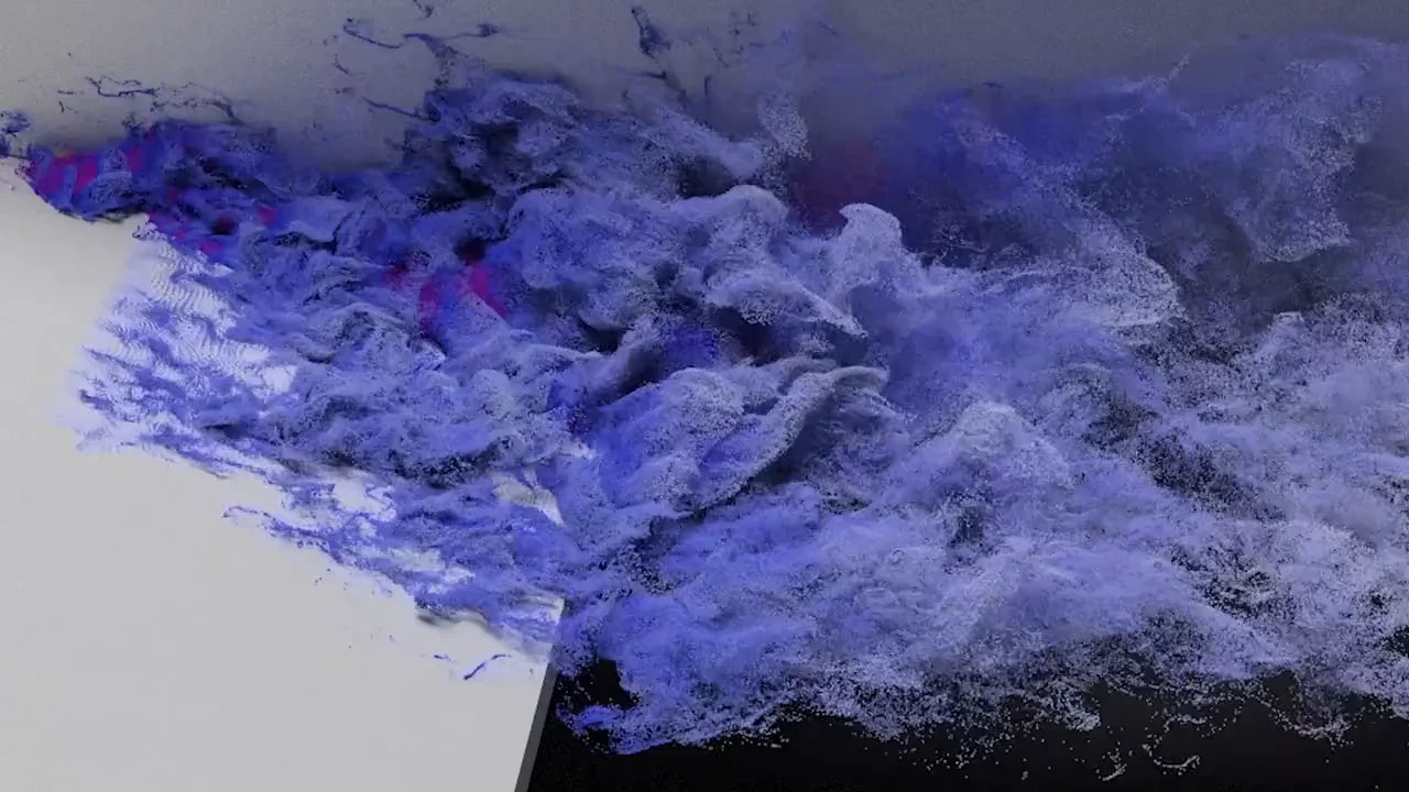
The same argument needs rechecking whenever the mesh, time step, material coefficients or boundary conditions change, because those can change the operator itself. Some stages also depend on more than the local update suggests. An incompressible flow solver, for example, couples pressure and velocity through a pressure equation, which the OpenFOAM documentation describes for the SIMPLE and PISO algorithms. The NASA jet above is a visualization of aerodynamic flow from NASA’s computational fluid dynamics work. It shows the kind of data a simulation produces, while the heat example isolates the dependency pattern.

Change propagation does not always win. The experimental analysis of self-adjusting computation by Acar and colleagues notes that large asymptotic speedups from propagating changes are uncommon, even though the method can update a computation as if the program had been rerun from scratch. Treat the speedup as a result to measure on your own operator.

Compare the whole run with the reference

Pick one frequently called operator and record how its inputs change on a representative run. Compare a full application with a version that updates the prior result, using the same precision, stopping criteria and hardware. Check agreement at intermediate steps and on the final quantities you use to make decisions, such as a peak temperature, a force or a residual.

Measure time to solution and, when available, energy per completed run. Include the time to detect changes, maintain state and return to a full evaluation on a broad update. Repeat the comparison for a local perturbation, a burst of changes and a case where most inputs change. That is enough to tell whether this operator is worth pursuing on this workload.

Sources

• Oxford numerical methods notes on the finite-difference heat equation
• Rutgers lecture notes on finite-difference schemes for the heat equation and their stability
• PETSc documentation for matrix-vector products
• OpenFOAM documentation for pressure-velocity coupling
• Acar, Blelloch, Blume, Harper and Tangwongsan, an experimental analysis of self-adjusting computation (ACM TOPLAS)
• Differential dataflow
• NASA Ames jet-flow visualization